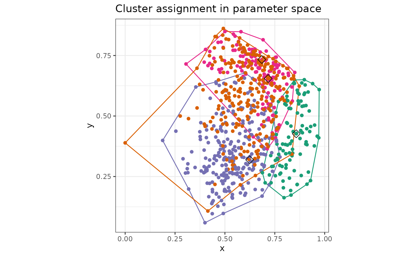
Generate a specified plot outside the GUI
makePlots.RdAn interface to generate a specific graph seen when using the GUI. Settings include: metric, linkage, k, plotType, for details see the vignette on using this function.
Usage
makePlots(
  cluster,
  settings,
  cov = NULL,
  covInv = NULL,
  exp = NULL,
  linked = NULL,
  linked.cov = NULL,
  linked.covInv,
  linked.exp = NULL,
  user_dist = NULL,
  getCoordsSpace1 = normCoords,
  getCoordsSpace2 = normCoords,
  getScore = NULL,
  results = NULL
)
Arguments
- cluster
dataframe of variables in cluster space
- settings
list specifying parameters usually selected in the app
- cov
covariance matrix for space 1
- covInv
inverse covariance matrix for space 1
- exp
reference point in space 1
- linked
dataframe of variables in linked space
- linked.cov
covariance matrix for space 2
- linked.covInv
inverse covariance matrix for space 2
- linked.exp
reference point in space 2
- user_dist
user defined distances
- getCoordsSpace1
function to calculate coordinates in cluster space
- getCoordsSpace2
function to calculate coordinates in linked space
- getScore
function to calculate scores and bins
- results
an output of
makeResults(), used to reduce computation when many plots are made.
Examples
makePlots(
cluster = Bikes$space1,
settings = list(
plotType = "WC", x = "hum", y = "temp", k = 4, metric = "euclidean",
linkage = "ward.D2", WCa = 0.5, showalpha = TRUE
), cov = cov(Bikes$space1),
linked = Bikes$space2, getScore = outsideScore(Bikes$other$res, "Residual")
)
 makePlots(
cluster = Bikes$space1,
settings = list(
plotType = "tour", k = 4, metric = "euclidean", linkage = "ward.D2",
tourspace = "space1", colouring = "clustering", out_dim = 2, tour_path = "grand",
display = "scatter", radial_start = NULL, radial_var = NULL, slice_width = NULL, seed = 2025
),
cov = cov(Bikes$space1), linked = Bikes$space2,
getScore = outsideScore(Bikes$other$res, "Residual")
)
makePlots(
cluster = Bikes$space1,
settings = list(
plotType = "tour", k = 4, metric = "euclidean", linkage = "ward.D2",
tourspace = "space1", colouring = "clustering", out_dim = 2, tour_path = "grand",
display = "scatter", radial_start = NULL, radial_var = NULL, slice_width = NULL, seed = 2025
),
cov = cov(Bikes$space1), linked = Bikes$space2,
getScore = outsideScore(Bikes$other$res, "Residual")
)